Let’s start with the distribution of colors in a picture.

The color distribution reflects how the pixels are colored. In the space of RGB(red, green, blue), each pixel is represented by 24 bits (8 bits for red, 8 for green and 8 for blue). For example, given 8 bits to describe how red it is, there are 256 ($2^8$) different variations. In total, there are 16,777,216 ($256^3$) different kinds of RGB combinations, which already reaches the limit of human eyes.

To find similar images, the basic idea is that similar images share similar color distributions. To quantify similarities, it’s straightforward to make use of pixel counts to build up the profiles, which we call signatures.

Signatures

Let’s start with a simple example, assume that we partition each color into two categories:

• not-so-red vs red
• not-so-green vs green
• not-so-blue vs blue

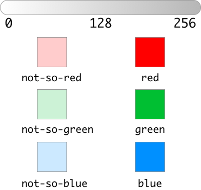
All the pixels are partitioned into 8 ($2^3$) categories, and the pixel counts should be a list with 8 integers:

pixelCounts = [0, 0, 0, 0, 0, 0, 0, 0]

For example, if the first pixel has a RGB value of (150, 20, 30), it be considered as (red, not-so-green, not-so-blue), and thus we increase the bucket 1,0,0 by 1.

pixelCounts[4] += 1

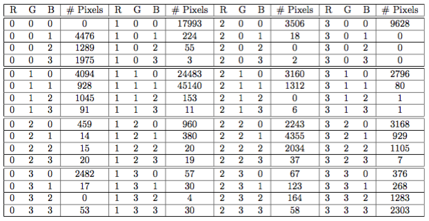
After walking through all the pixels in the image,

pixelCounts = [0, 6197, 0, 0, 7336, 15, 4961, 0]

The list pixelCounts contains the information about color distributions, and we call it a signature.

When we hash all colors into several buckets, it is intuitional to see similar colors in the same bucket. For example, 150, 20, 30 and 155, 22, 35 are very similar, so both of them are put into the same bucket.

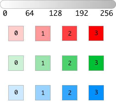
If we increase the number of buckets, the signatures will be longer. For example, a 4-segmented signature contains 64 ($4^3$) integers.

Similarities

Now we extract a signature for every picture, the next job is to find how to measure the similarities between the signatures.

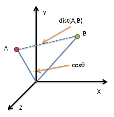
Cosine Similarity is an inner product space that measures the cosine of the angle between them. The figure above illustrates that Cosine Similarity measures the angle between the vector space, compared to Euclidean Distance (a measure of the absolute distance between two points), more is to reflect differences in direction, but not the location.

If consider the signatures as 64-dimensional vectors, we could use Cosine Similarity to quantify their similarities.

Locality Sensitive Hashing

Locality Sensitive Hashing (LSH) is an algorithm for searching near neighbors in high dimensional spaces. The core idea is to hash similar items into the same bucket. We will walk through the process of applying LSH for Cosine Similarity, with the help of the following plots from Benjamin Van Durme & Ashwin Lall, ACL2010, with a few modifications by me.

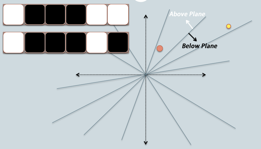
1. In the Figure 1, there are two data points in red and yellow, representing two-dimensional data points. We are trying to find their cosine similarity using LSH.
2. The gray lines are randomly picked planes. Depending on whether the data point locates above or below a gray line, we mark this result as $1$ (above the line, in white) or $0$ (below the line, in black).
3. On the upper-left corner, there are two rows of white/black squares, representing the results of the two data points respectively.

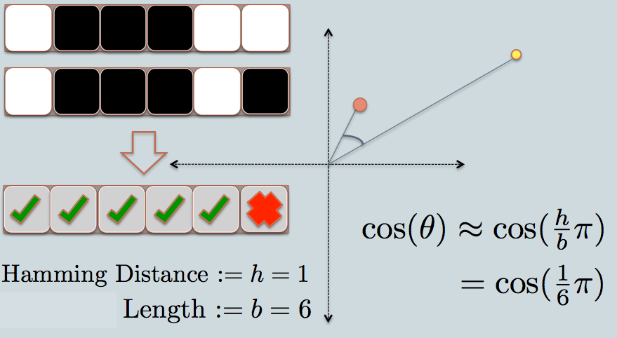
1. As in the example, we use 6 planes, and thus use 6 bits to represent each data. The length of sketch $b = 6$.
2. The hamming distance between the two hashed value $h = 1$.
3. The estimated cosine similarity is $cos(\frac{h}{b}\pi)$.

These randomly picked planes are used as the buckets to hash the data points. We are able to estimate the cosine similarities from the hamming distances, the calculation of latter relatively more efficient.

Cosine Similarity is not sensitive to the magnitude of vectors. In some scenarios, people will apply Adjusted Cosine Similarity to reduce such sensitivity. Since the only concern here is to find whether the data points are located at the same side of the plane, there is no need to adjust the vectors, before calculating their similarities.

We can consider the pool of $k$ random planes playing the role of the hash function. Random planes are easy to generate, and highly efficient to apply in matrix.

Sketches

As we apply $k$ random planes to the whole dataset, each data point generates a $k$-bit vector, we call such vector as a sketch.

from numpy import zeros, random, dot

def sketch(M, k):

    '''
    M: the matrix of signatures.
    k: random vector counts.
    '''
    w,h = M.shape

    # generating k random directions. use vectors
    # of normally distributed random numbers.
    rd = random.randn(k, h)

    # init sketches
    sketches = zeros((k, w))

    # for each random plane
    for i in range(k):
        # for each signature
        for j in range(w):
            # whether the data point is above the random plane
            v = dot(rd[i], M[j])
            if v > 0:
                sketch = 1
            elif v < 0:
                sketch = 0
            # v == 0 is of a tiny probability, choose 1 or 0 randomly
            else:
                if random.random() >= 0.5:
                    sketch = 1
                else:
                    sketch = 0
            sketches[i][j] = sketch
    return sketches

Let’s walk through all these steps before moving to the nearest neighbors:

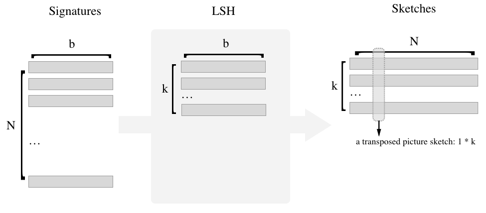
• Signature
  • The image dataset contains $N$ pictures. (e.g, $N = 100,000$)
  • Color spaces are cut into $b$ buckets. (e.g, $b = 64$)
  • Each signature thus consists of $b$ integers.
  • The shape of signature matrix is N * b. ($N$ rows, $b$ columns)

• LSH
  • The LSH family contains $k$ random vectors. (e.g, $k = 256$)
  • Each random vector is of $b$ dimension, abd thus has $b$ random floats.
  • The shape of random vector matrix is k * b.

• Sketch
  • For each random plane, calculate whether the data points are above it.
  • Entries of the sketch matrix are binary.
  • The shape of sketch matrix is k * N.

Nearest Neighbors

In order to find the nearest neighbors for a given picture, we can calculate the hamming distance in naive loops.

def nested_loop(sketches, line):
    '''Naive method to calculate hamming distance'''
    h,w = sketches.shape
    r = []
    for i in range(0, w):
        intersection = 0
        for k in range(0, h):
            if sketches[k][i] == sketches[k][line]:
                    intersection += 1
        r.append(round(
            float(intersection) / float(w),
            4
        ))
    return r

The naive method uses nested loop to calculate hamming distance, which causes inefficiency for big matrices.

It’s intuitive to use matrix-friendly method since we could have millions pictures.

A better method is to select the corresponding row of transposed sketch matrix, which stands for the binary relations between the given picture and $k$ random planes.
Then calculate dot product of picture sketch 1 * k and matrix k * N, which is a 1 * N array of integers.
We would like to make this 1 * N array, highly correlated to the collection of hamming distances between the given picture and all.

>>> import numpy as np

>>> a1 = np.array([ 0, 1, 1, 0])
>>> b1 = np.array([ 1, 0, 1, 0])

>>> a1 ^ b1
array([1, 1, 0, 0])
# the hamming distance between a1 and b1 is 2

>>> sum(a1 ^ b1)
2
# min distance is 0, and max is 4

To speed up the calculation, we replace all $0$ with $-1$.
Since,
$$ (-1) * (-1) = 1 * 1 = 1 $$
And,
$$ 1 * (-1) = (-1) * 1 = -1 $$
The dot product of new sketch will be an integer between $[-k, k]$.
Higher dot product indicates higher similarity, because each similar part contributes $1$ to the result and dissimilar one contributes $-1$.

>>> a2 = np.array([-1, 1, 1,-1])
>>> b2 = np.array([ 1,-1, 1,-1])
>>> np.dot(a2, b2)
0
# (-1)*1 + 1*(-1) + 1*1 + (-1)*(-1) = 0.
# min dot is -4, and max is 4

It’s easy to prove that Dot Product(DP) is directly proportional to the Hamming Distance(HD):

$$ DP_{A,B} = Sketch_A * Sketch_B’ = N_{same} - N_{diff} $$

Since, $$ N_{same} + N_{diff} = k $$

Finally, $$ HD_{A,B} = \frac{N_{same}}{k} = \frac{ DP_{A,B} + k }{2} * \frac {1}{k} = \frac{DP_{A,B}}{2k} + \frac{1}{2} $$

The function is as follows:

def similar(sketches, line):

    def transpose_dot(sketches, line):
        result = dot(sketches.transpose()[line], sketches)
        return result

    scores = transpose_dot(sketches)

    n = 20
    top_n = argsort(scores)[-n:][::-1]
    #       argsort(scores)[-n:]       # last n elements
    #                           [::-1] # reverse to get top N lines
    return top_n

By reversing the list of scores, we select best $n$ candidates according to descending scores.

Tuning Parameters

Tuning parameters to find the optimum balance between accuracy and efficiency is important in the implementation.

For example, in general, the r-squared of sketch similarity and signature similarity rises with number of vectors. More random vectors can provide better estimation of the similarity, but at the same time cost more time and memory. Thus experiments are carried out as follows:

From the above graphs, we can select $k=256$ to get a r-squared greater than $0.9$ while keeping efficiency.

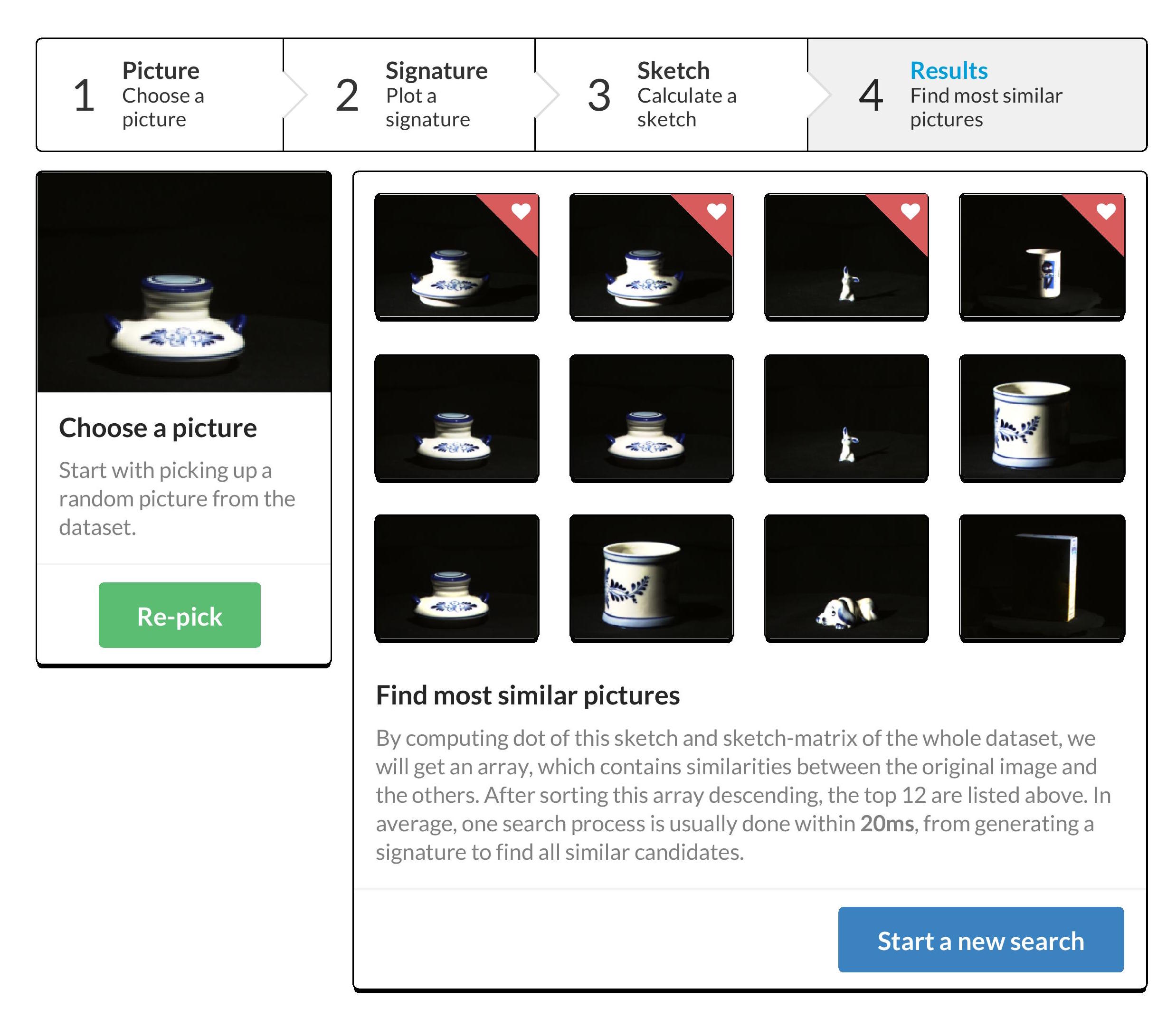
Demo

I made a side project called Prism.
Prism provides a web-based interface to explain the process from extracting features to searching nearest neighbors.
It contains not only the implementation of above algorithms, also uses a dataset with 24,000 pictures as a full-function demo.

All the source codes, datasets, results and analysis are in the github repository github.com/kainliu/Prism.

1	2

3	4

Experiements

1	2

3	4

As we seen from the above results - nearest neighbors have similar colors - which basically fits our original idea.

Wrapping Up

It’s a meaningful trial for me, to starting from an idea to presenting a viable tool.

However, this method is highly influenced by the diversity of colors. For example, the 4th experiment mixed the pictures of white cups with the baseballs, since they share a large percentage of similar white colors.

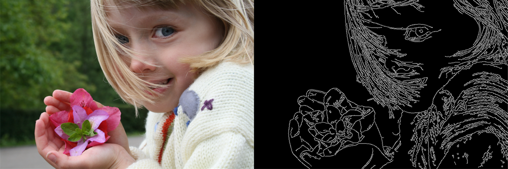
To overcome this shortcoming, an option is to take boundaries of the objects into account. There are many popular algorithms in contour/edge detection.